How Condatis works

Overall concept

Condatis offers a way of assessing a habitat network – a map of habitat is the main input – by quantifying how quickly a species can shift its range through the network. The speed of range shifting is not the same as the speed of individual dispersal movements. The habitat in Condatis drives species’ reproduction as well as providing stepping stones for movement.

What does Condatis do?

• Highlights pathways that allow both dispersal and population growth of species as they cross a landscape.
• Pinpoints bottlenecks in the habitat network (where there are restricted opportunities for colonisation).
• Ranks the feasible sites for habitat creation and restoration to enhance the existing habitat network efficiently.

Check out our page ‘What can I get out of Condatis’, if you want a short, non-technical overview of why conservation practitioners find Condatis useful. What follows below is a slightly more detailed explanation of how Condatis works.

“We are working with ‘open water’ (mostly ponds and lakes) in the northern upland chain LNP.  Ponds (and water) is a good one, we thought, because it is easy to target new habitat through working with farmers and the stewardship schemes. We are really pleased with Condatis.”
A. Mansley, Senior Environment Analyst, Northumberland National Park Authority

The scenario of range expansion

To expand its range, a species must repeatedly colonise and establish populations in new sites. The main factors affecting the speed of range expansion are:

1. The rate of reproduction, which enhances the total number of emigrant individuals leaving existing populations.
2. The dispersal distances of the emigrant individuals – further is almost always better, especially if the landscape is fragmented. (In Condatis the dispersal distances are statistically described by a negative-exponential distribution, sometimes called a “dispersal kernel”).
3. The availability of empty habitat patches to land in.

Condatis puts these three key factors together into a relatively simple but powerful model.

Imagine a patchy landscape with your species of interest initially occupying one margin, or even one site. We term this initially populated habitat the SOURCE. You are interested in how long it would take for some descendants of that population to colonise the other end of the landscape – we term this area the TARGET.

To colonise the TARGET, we probably need to wait for a long chain of colonisation events, and multiple generations, as the species progresses from patch to patch and builds up populations. It is difficult to predict in what order these colonisations will happen – there is randomness involved. And the more patches the landscape contains, the more possible orderings there are.

Luckily, though, we can predict the “waiting time” for each single colonisation step. We use the dispersal and reproduction information for every pair of patches to ask “if patch A was occupied, how long would it take to send a colonist to hit patch B”?

Next, we convert the waiting times into RESISTANCE values, as if the habitat network were an electrical circuit. Circuit theory turns out to be extremely helpful to predict the overall average properties of the habitat network, without running through the countless possible orderings mentioned above.

Resistance, time and flow

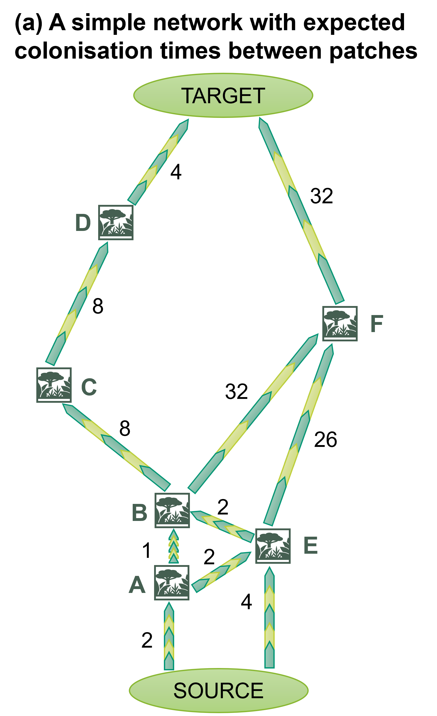
The figure below on the left, diagram (a), shows a few habitat patches linked together by waiting times. For example, the total mean time from the source to the target going via A-B-C-D is 23 generations, whereas going via E-F it takes 62 generations.

In a circuit, you may be familiar with the idea that current takes the route of least resistance. In fact, it’s truer to say that current flow is shared out over the available routes, with the lowest-resistance routes taking most of it.

Because we have equated resistance with the time taken until colonisation, it turns out that the routes with high current flow in the circuit analogy are the quickest routes for the species in the ecological scenario.

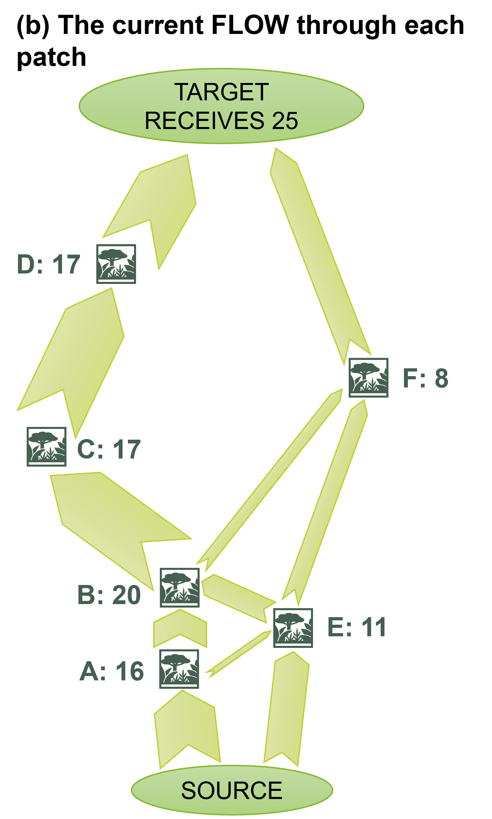
This may sound odd, but it becomes easier to understand when you look at Condatis outputs showing the FLOW through different patches (habitat-containing raster cells) between the SOURCE and the TARGET.

The FLOW that arises from the resistance values on the left diagram (a) is shown on the right (b). We see that patch B has the highest FLOW.

The sum of FLOW that arrives at the TARGET is our overall metric of SPEED, which summarises how quickly the TARGET can be colonised, starting from the SOURCE. In the diagram below, SPEED is 25. In 2012 we showed that SPEED is well correlated to the speed of range expansion in a simulated population (Hodgson et al, 2012), and in 2022, we showed that it is also a helpful predictor of real range expansions in UK moth species (Hodgson et al, 2022).

The larger the flow value of a habitat cell, the more important that cell is for connectivity between the source and the target. Cells with high flow are priorities for conservation because, if they were lost, the overall speed is likely to suffer (these costs of loss were demonstrated in Hodgson et al, 2016).

Bottlenecks – where flow is restricted

The other major output of a Condatis analysis is the BOTTLENECKS lines. Bottlenecks help you to identify the places where additional habitat would be most beneficial to range-shifting speed. A place is a bottleneck if it has high resistance and yet forms part of one of the best available routes through the landscape. If habitat were added on or around the lines representing these bottleneck links, then the whole route would have significantly higher flow (these large marginal changes were demonstrated in Hodgson et al, 2016). Therefore, the map of the top bottleneck links gives suggestions of where you would ideally add habitat, if you could only make one change to the network.

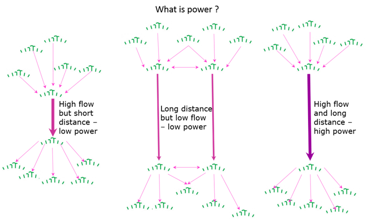
Getting a bit more technical, the BOTTLENECK strength is defined as the electrical power lost from a link in the circuit. Power combines current and resistance, in such a way that it highlights where a link carries disproportionately high FLOW considering its high RESISTANCE. The below diagram helps to explain this, but also, seeing the location of bottlenecks in your own data usually makes intuitive sense.

Is this the right software for me?